STEP #3 - ANALYZE CON’T
ORGANIZE & ANALYZE DATA


© The Quality Web, authored by Frank E. Armstrong, Making Sense Chronicles - 2003 - 2016


Step #3 - ANALYZE - PART .3
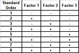
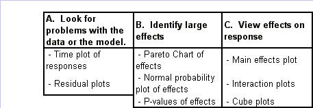
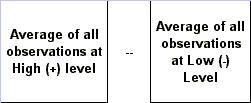
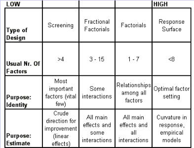
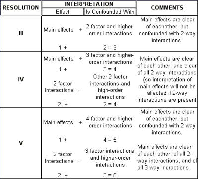
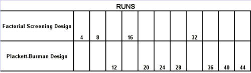
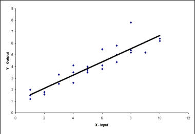
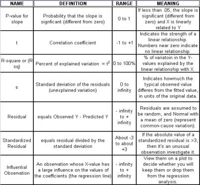
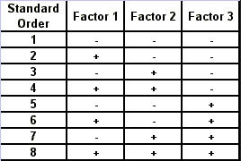
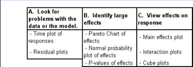
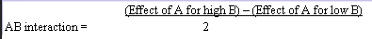
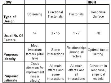
Regression Analysis Regression analysis generates a line that quantifies the relationship between X and Y. The line, or regression equation, is represented as Y = b0 + b1X, where b0 = intercept (where the line crosses X - 0); b1 = slope (rise over run, or change in Y per unit increase in X). Benefits of quantifying a relationship · Prediction - The equation can be used to predict future Ys by plugging in an X-value. · Control - If X is controllable, you can manipulate process conditions to avoid undesirable results and/or generate desirable results. Extrapolation is making predictions outside the range of the X data. It is a natural desire, but it is like walking down from solid ground onto thin ice. Predictions from regression equations are more reliable for Xs within the range of observed data. A residual is the vertical distance from each point to the regression line. It equals Observed Y minus Predicted Y. It is the leftover variation in Y after using X to predict Y. The Least Squares Method The regression equation is determined by a procedure that minimizes the total squared distance of all points to the line. · Finds the line where the squared vertical distance from each data point to the line is as small as possible (or the "least"). · Restated…minimizes the "square" of all the residuals. · Regression uses the least squares method to determine the "best line": o Data (both X and Y values) are used to obtain b0 and b1 values. o The b0 and b1 values establish the equation. Assumptions of regression are based on properties of the residuals (not the original data). We assume residuals are: · Not related to the Xs. · Stable and Independent, do not change over time. · Constant, do not increase as predicted Ys increase. · Normal (bell-shaped) with mean of 0. · Residuals vs. Each X is used to check that the residuals are not related to the Xs - if the relationship between X and Y is not a straight line, but a curve, try a transformation on X, Y, or both. Or use X2 in a multiple regression. · Residuals vs. Predicted Y (Fits) is used to check that they are constant over the range of Ys. - a fan shape means the variation increases as Y gets larger (it's not constant). Try a square root, log, or inverse transformation on Y. · Normal Probability Plot of Residuals is used to check that residuals are Normal - If the residuals are not Normal, try a transformation on X or Y or both. Confidence and Prediction Intervals · Confidence Interval - An interval likely to contain the "best fit" line. It gives a range of the predicted values for the fitted Y if the regression is repeated again. It is based on a given X-value for a given confidence. · Prediction Interval - An interval likely to contain the actual Y values for a given X. It gives a range of likely actual values for Y, is based on a given X-value, and is for a given Confidence interval. · A Confidence interval, which is predicting how much he fitted line could vary, will always be narrower than a Prediction Interval, which accounts for variation of the individual values around the fitted line. DESIGN OF EXPERIMENTS Design of Experiments is an approach for effectively and efficiently exploring the cause- and-effect relationship between numerous process variables (Xs) and the output or process performance variable (Y). It identifies the "vital few" sources of variation (Xs) - those that have the largest impact on the output results; it quantifies the effects of the important Xs, including their interactions; and it produces an equation that quantifies the relationship between the Xs and Y. From that y ou can predict how much gain or loss will result from the changes in process conditions. There are several methods in use out there to include my favorite, the Taguchi method. We will, however, cover the basic or generic method here. Full Factorial The Factorial Approach to Designed Experiments: · Changes several factors (variables) simultaneously, not one at-a-time. · Initially begins with only 2 conditions of factor conditions. · Considers all possible combinations of factor conditions. · May test all the combinations or a carefully selected sub-set of them. · Handles random (common-cause) variation easily and uses it to determine which factors are important. · Replication of trials (repeated testing of same combinations) is encouraged to help measure common-cause variation. · Is easy to analyze. · Uses methods to deal with other factors not controlled in the experiment (such as randomization and blocking) so that conclusions are still valid. A full factorial involves all possible combinations. For 3 factors, each at 2 levels, there are 2 x 2 x 2 = 8 combinations of factor settings. 2 x 2 x 2 is often written as 23 with the superscript 3 indicating the number of levels (2s) multiplied together. For 3 factors, there are 8 possible combinations of factor settings. An example layout is created below. Designing a full factorial experiment: Replication means repeating all the experimental conditions two or more times. Why do replicates? · To measure pure error: the amount of variability among runs performed at the same experimental conditions (this will represent common cause variation). · To see more clearly whether or not a factor is important - is the difference between responses due to a change in factor conditions (an induced special cause) or is it due to common cause variability? · To see the effect of changing factor conditions not only on the average response, but also on response variability, if desired (two responses can be analyzed: the mean and the standard deviation). Randomization Definition: · To assign the order in which the experimental trials will be run using a random mechanism. · It is not the standard order. · It is not running trials in an order that is convenient. · To create a random order, you can "pull numbers from a hat" or have a computer randomize the sequence of trials for you. Why? · Averages the effect of any lurking variables over all of the factors in the experiment. · Prevents the effect of a lurking variable from being mistakenly attributed to another factor. · Helps validate statistical conclusions made from the experiment. Analyzing the Experiment There are basically three phases of data analysis; they are: Look for problems with the data. 1. Make a time plot of the response. 2. Interpret the plot by looking for: a. "Defects" in the data such as missing values, typo's, and so forth. b. Trends or cycles that indicate lurking variables associated with time. Residuals Definition: Residual = (Observed Y) - (Average of Ys at that experimental condition). A residual is the difference between a response and what we "expect" it to be (the expected value is the average of all replicates for a particular combination of factor settings). We hope that most variation in the Ys is accounted for by deliberate changes we're making in the factor settings. Whatever variation is left over is residual - the assumption is that this residual variation reflects the common cause-variation in the experiment. Assumptions of DoE Analysis The Residuals: Residual: Residual = (Observed Y) - (Average at each experimental condition) We assume the residuals are: · Normal - bell-shaped with a mean of 0. · Constant - do not increase as averages of each experimental condition increases. · Stable - do not change over time. · Not related to the Xs (factors). · Random - represent common causes of variation. · Independent Residual plots must be checked to ensure the assumptions hold. Otherwise, conclusions could be incorrect and thus misleading. Once you have verified that there are no problems with the data, you can look for factors that have the largest effect on the response. There are two types of effects, main effects and interaction effects. Main Effect Definition - the main effect is the average increase (or decrease) in the response when moving from the low to the high level of a factor. The Formula for calculating main effects for each factor is: A hypothesis test: · Tests the "null" hypothesis (no difference between groups). · Against the alternative hypothesis (groups are different). · Obtain a P-value for the null hypothesis. · Use the data and the appropriate hypothesis; test statistic to obtain a P-value. · If P is less than .05, reject the H0 and conclude the Ha. · If P is greater than or equal to .05, cannot reject the H0. Interaction Effects Definition - an interaction occurs when the effect one factor has on the response (Y) is not the same for each level of another factor. Formula for calculating the size of interaction effects is: Deciding which effects are large (or significant). There are three ways to decide which effects are large: · P-value for each effect · Pareto chart of effects · Normal probability plot of effects. Drawing conclusions · List all your conclusions · Interpret the meaning of these results · Make recommendations · Formulate and write conclusions in simple language. The Prediction Equation - using coefficients Use the coefficients to generate an equation that lets you predict the response (Y) for various combinations. Say for example, for just one numerical factor, suppose the uncoded effect of A would be .34. The prediction equation for Y then is Y = Constant + .34A. Dropping terms from the prediction equation Remove the insignificant terms. If an interaction is significant, it is standard practice to include the main effects of the factors involved, even if the main factors by themselves aren't significant. Verify Results There are two key ways to verify the conclusions drawn from an experiment: · Confirmatory runs - run a few additional experiments at the recommended settings to see if the desired response is achieved. Can you turn it on and turn it off? · Make actual recommended process changes - Change the process and monitor it on a control chart to assure that the desired response is achieved and maintained. Reducing Experimental Trials - The Half-Fraction and confounding · In a full factorial design, information is available for all main effects. · Interactions - Two-factor (AB, AC, or BC). Higher order interactions for three or more factors (ABC, ABCDF, ADED). · When there are many factors, the number of higher-order interactions increases quickly. · Higher-order interactions are usually negligible (involving more than 2 factors). · There is a diminishing return of information on higher-order interactions; in general, the higher-order they are, the more negligible. Cost/benefit of a half-fraction for 5 factors COST - Main effects and two-factor interactions are confounded with higher-order interactions. BENEFIT - The number of runs is reduced by half. Reduced Fractional Designs The knowledge line is a strategy for choosing the appropriate design. Which approach to designed experiments you choose depends on how much you already know about a process and how many factors you want to test. The chart below is offered to lend some guidance: The "cost" of running fractional factorials is that effects and interactions will be confounded. The resolution (indicated by the Roman numerals above) describes the degree of confounding; the higher the number, the more resolution ( = less confounding). A resolution V design has less confounding than a resolution III. Resolution tells us the type of effects that will be confounded. SCREENING DESIGNS: · They study the main effects of a large number of factors. · They contain roughly the same number of runs as factors. · They are resolution III. · They are useful in the early stages of investigation when it is desirable to go from a large list of factors that may affect the response to a small list of factors that actually do affect the response. Tips for the analysis of screening designs: · Check the confounding results carefully. · An important effect labeled C, for instance, could also be the result of several 2- factor interactions. · Analyze the collapsed design. · If only factors A, F, and G turn out to be important, drop the other factors and analyze the design again. PLACKETT-BURMAN DESIGNS These designs follow a special pattern of confounding to let you reduce the number of runs needed. Plackett-Burman designs are available for 4 (i) runs where "i" is an integer. When to use Plackett-Burman Designs: · Use them when it is too costly to run the 2k (8-, 16-, or 32- run) screening design. · Use them only in these circumstances, because the "cost" of this design is the loss of information about where the 2-factor interactions are confounded. Summary of fractional factorials and screening designs: · Much of the information obtained in a full factorial can be obtained using only a faction of the full factorial. · Screen designs can be used to screen a large number of factors in a few runs to determine which are important. In screening designs, main effects are confounded with 2-factor interactions (resolution III). · Other fractional factorials are useful in situations where it is important to understand which factors and interactions affect the response. · Resolution tells us which effects are confounded. · Plackett-Burman designs can be used in screening situations where 16 or 32 runs are too costly. FULL FACTORIALS WITH MORE THAN TWO LEVELS Full Factorial Designs can be constructed for any number of factors with any number of levels. When there are more than two levels, they provide all the benefits of the Factorial designs, as well as the Response Surface Designs. Full Factorial Designs often have many runs. For example, a design with the below has 30 runs: 1 factor at 2 levels. 1 factor at 3 levels 1 factor at 5 levels This design is particularly useful when you want to study a factor that it is difficult to represent with 2 levels. For example, if there are multiple machines used in production, you may want to understand the behavior of all of them, not just two of them. Planning and Preparing for a Design of Experiment Before the Experiment: A. Preliminaries B. Identifying responses, factors and factor levels. C. Selecting the design. During the Experiment D. Collecting the Data After the Experiment: E. Analyzing the data. F. Drawing, verifying, and reporting conclusions. G. Implementing recommendations. COMPLETION CHECKLIST: Upon completing this ANALYZE phase, you should be able to now approach the IMPROVE phase since you have learned: · Which potential causes you identified · Which potential causes you decided to investigate and why · What data you collected to verify those causes · How you interpreted the data. THIS IS THE END OF THE ANALYZE PHASE - GO BACK TO SIX SIGMA PAGE AND START IMPROVE PHASE TO CONTINUE LEARNING ABOUT SIX SIGMA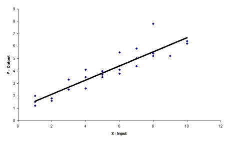

RESOLUTION: UNDERSTANDING THE DEGREE OF CONFOUNDING IN A FRACTIONAL FACTORIAL


STEP #3 - ANALYZE CON’T
ORGANIZE & ANALYZE DATA

Step #3 - ANALYZE - PART .3
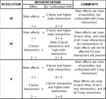
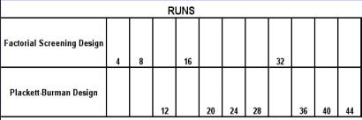
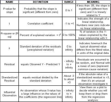
Regression Analysis Regression analysis generates a line that quantifies the relationship between X and Y. The line, or regression equation, is represented as Y = b0 + b1X, where b0 = intercept (where the line crosses X - 0); b1 = slope (rise over run, or change in Y per unit increase in X). Benefits of quantifying a relationship · Prediction - The equation can be used to predict future Ys by plugging in an X-value. · Control - If X is controllable, you can manipulate process conditions to avoid undesirable results and/or generate desirable results. Extrapolation is making predictions outside the range of the X data. It is a natural desire, but it is like walking down from solid ground onto thin ice. Predictions from regression equations are more reliable for Xs within the range of observed data. A residual is the vertical distance from each point to the regression line. It equals Observed Y minus Predicted Y. It is the leftover variation in Y after using X to predict Y. The Least Squares Method The regression equation is determined by a procedure that minimizes the total squared distance of all points to the line. · Finds the line where the squared vertical distance from each data point to the line is as small as possible (or the "least"). · Restated…minimizes the "square" of all the residuals. · Regression uses the least squares method to determine the "best line": o Data (both X and Y values) are used to obtain b0 and b1 values. o The b0 and b1 values establish the equation. Assumptions of regression are based on properties of the residuals (not the original data). We assume residuals are: · Not related to the Xs. · Stable and Independent, do not change over time. · Constant, do not increase as predicted Ys increase. · Normal (bell-shaped) with mean of 0. · Residuals vs. Each X is used to check that the residuals are not related to the Xs - if the relationship between X and Y is not a straight line, but a curve, try a transformation on X, Y, or both. Or use X2 in a multiple regression. · Residuals vs. Predicted Y (Fits) is used to check that they are constant over the range of Ys. - a fan shape means the variation increases as Y gets larger (it's not constant). Try a square root, log, or inverse transformation on Y. · Normal Probability Plot of Residuals is used to check that residuals are Normal - If the residuals are not Normal, try a transformation on X or Y or both. Confidence and Prediction Intervals · Confidence Interval - An interval likely to contain the "best fit" line. It gives a range of the predicted values for the fitted Y if the regression is repeated again. It is based on a given X-value for a given confidence. · Prediction Interval - An interval likely to contain the actual Y values for a given X. It gives a range of likely actual values for Y, is based on a given X-value, and is for a given Confidence interval. · A Confidence interval, which is predicting how much he fitted line could vary, will always be narrower than a Prediction Interval, which accounts for variation of the individual values around the fitted line. DESIGN OF EXPERIMENTS Design of Experiments is an approach for effectively and efficiently exploring the cause-and- effect relationship between numerous process variables (Xs) and the output or process performance variable (Y). It identifies the "vital few" sources of variation (Xs) - those that have the largest impact on the output results; it quantifies the effects of the important Xs, including their interactions; and it produces an equation that quantifies the relationship between the Xs and Y. From that y ou can predict how much gain or loss will result from the changes in process conditions. There are several methods in use out there to include my favorite, the Taguchi method. We will, however, cover the basic or generic method here. Full Factorial The Factorial Approach to Designed Experiments: · Changes several factors (variables) simultaneously, not one at-a-time. · Initially begins with only 2 conditions of factor conditions. · Considers all possible combinations of factor conditions. · May test all the combinations or a carefully selected sub-set of them. · Handles random (common-cause) variation easily and uses it to determine which factors are important. · Replication of trials (repeated testing of same combinations) is encouraged to help measure common-cause variation. · Is easy to analyze. · Uses methods to deal with other factors not controlled in the experiment (such as randomization and blocking) so that conclusions are still valid. A full factorial involves all possible combinations. For 3 factors, each at 2 levels, there are 2 x 2 x 2 = 8 combinations of factor settings. 2 x 2 x 2 is often written as 23 with the superscript 3 indicating the number of levels (2s) multiplied together. For 3 factors, there are 8 possible combinations of factor settings. An example layout is created below. Designing a full factorial experiment: Replication means repeating all the experimental conditions two or more times. Why do replicates? · To measure pure error: the amount of variability among runs performed at the same experimental conditions (this will represent common cause variation). · To see more clearly whether or not a factor is important - is the difference between responses due to a change in factor conditions (an induced special cause) or is it due to common cause variability? · To see the effect of changing factor conditions not only on the average response, but also on response variability, if desired (two responses can be analyzed: the mean and the standard deviation). Randomization Definition: · To assign the order in which the experimental trials will be run using a random mechanism. · It is not the standard order. · It is not running trials in an order that is convenient. · To create a random order, you can "pull numbers from a hat" or have a computer randomize the sequence of trials for you. Why? · Averages the effect of any lurking variables over all of the factors in the experiment. · Prevents the effect of a lurking variable from being mistakenly attributed to another factor. · Helps validate statistical conclusions made from the experiment. Analyzing the Experiment There are basically three phases of data analysis; they are: Look for problems with the data. 1. Make a time plot of the response. 2. Interpret the plot by looking for: a. "Defects" in the data such as missing values, typo's, and so forth. b. Trends or cycles that indicate lurking variables associated with time. Residuals Definition: Residual = (Observed Y) - (Average of Ys at that experimental condition). A residual is the difference between a response and what we "expect" it to be (the expected value is the average of all replicates for a particular combination of factor settings). We hope that most variation in the Ys is accounted for by deliberate changes we're making in the factor settings. Whatever variation is left over is residual - the assumption is that this residual variation reflects the common cause- variation in the experiment. Assumptions of DoE Analysis The Residuals: Residual: Residual = (Observed Y) - (Average at each experimental condition) We assume the residuals are: · Normal - bell-shaped with a mean of 0. · Constant - do not increase as averages of each experimental condition increases. · Stable - do not change over time. · Not related to the Xs (factors). · Random - represent common causes of variation. · Independent Residual plots must be checked to ensure the assumptions hold. Otherwise, conclusions could be incorrect and thus misleading. Once you have verified that there are no problems with the data, you can look for factors that have the largest effect on the response. There are two types of effects, main effects and interaction effects. Main Effect Definition - the main effect is the average increase (or decrease) in the response when moving from the low to the high level of a factor. The Formula for calculating main effects for each factor is: A hypothesis test: · Tests the "null" hypothesis (no difference between groups). · Against the alternative hypothesis (groups are different). · Obtain a P-value for the null hypothesis. · Use the data and the appropriate hypothesis; test statistic to obtain a P-value. · If P is less than .05, reject the H0 and conclude the Ha. · If P is greater than or equal to .05, cannot reject the H0. Interaction Effects Definition - an interaction occurs when the effect one factor has on the response (Y) is not the same for each level of another factor. Formula for calculating the size of interaction effects is: Deciding which effects are large (or significant). There are three ways to decide which effects are large: · P-value for each effect · Pareto chart of effects · Normal probability plot of effects. Drawing conclusions · List all your conclusions · Interpret the meaning of these results · Make recommendations · Formulate and write conclusions in simple language. The Prediction Equation - using coefficients Use the coefficients to generate an equation that lets you predict the response (Y) for various combinations. Say for example, for just one numerical factor, suppose the uncoded effect of A would be .34. The prediction equation for Y then is Y = Constant + .34A. Dropping terms from the prediction equation Remove the insignificant terms. If an interaction is significant, it is standard practice to include the main effects of the factors involved, even if the main factors by themselves aren't significant. Verify Results There are two key ways to verify the conclusions drawn from an experiment: · Confirmatory runs - run a few additional experiments at the recommended settings to see if the desired response is achieved. Can you turn it on and turn it off? · Make actual recommended process changes - Change the process and monitor it on a control chart to assure that the desired response is achieved and maintained. Reducing Experimental Trials - The Half-Fraction and confounding · In a full factorial design, information is available for all main effects. · Interactions - Two-factor (AB, AC, or BC). Higher order interactions for three or more factors (ABC, ABCDF, ADED). · When there are many factors, the number of higher-order interactions increases quickly. · Higher-order interactions are usually negligible (involving more than 2 factors). · There is a diminishing return of information on higher-order interactions; in general, the higher-order they are, the more negligible. Cost/benefit of a half-fraction for 5 factors COST - Main effects and two-factor interactions are confounded with higher-order interactions. BENEFIT - The number of runs is reduced by half. Reduced Fractional Designs The knowledge line is a strategy for choosing the appropriate design. Which approach to designed experiments you choose depends on how much you already know about a process and how many factors you want to test. The chart below is offered to lend some guidance: The "cost" of running fractional factorials is that effects and interactions will be confounded. The resolution (indicated by the Roman numerals above) describes the degree of confounding; the higher the number, the more resolution ( = less confounding). A resolution V design has less confounding than a resolution III. Resolution tells us the type of effects that will be confounded. SCREENING DESIGNS: · They study the main effects of a large number of factors. · They contain roughly the same number of runs as factors. · They are resolution III. · They are useful in the early stages of investigation when it is desirable to go from a large list of factors that may affect the response to a small list of factors that actually do affect the response. Tips for the analysis of screening designs: · Check the confounding results carefully. · An important effect labeled C, for instance, could also be the result of several 2- factor interactions. · Analyze the collapsed design. · If only factors A, F, and G turn out to be important, drop the other factors and analyze the design again. PLACKETT-BURMAN DESIGNS These designs follow a special pattern of confounding to let you reduce the number of runs needed. Plackett-Burman designs are available for 4 (i) runs where "i" is an integer. When to use Plackett-Burman Designs: · Use them when it is too costly to run the 2k (8-, 16-, or 32- run) screening design. · Use them only in these circumstances, because the "cost" of this design is the loss of information about where the 2-factor interactions are confounded. Summary of fractional factorials and screening designs: · Much of the information obtained in a full factorial can be obtained using only a faction of the full factorial. · Screen designs can be used to screen a large number of factors in a few runs to determine which are important. In screening designs, main effects are confounded with 2-factor interactions (resolution III). · Other fractional factorials are useful in situations where it is important to understand which factors and interactions affect the response. · Resolution tells us which effects are confounded. · Plackett-Burman designs can be used in screening situations where 16 or 32 runs are too costly. FULL FACTORIALS WITH MORE THAN TWO LEVELS Full Factorial Designs can be constructed for any number of factors with any number of levels. When there are more than two levels, they provide all the benefits of the Factorial designs, as well as the Response Surface Designs. Full Factorial Designs often have many runs. For example, a design with the below has 30 runs: 1 factor at 2 levels. 1 factor at 3 levels 1 factor at 5 levels This design is particularly useful when you want to study a factor that it is difficult to represent with 2 levels. For example, if there are multiple machines used in production, you may want to understand the behavior of all of them, not just two of them. Planning and Preparing for a Design of Experiment Before the Experiment: A. Preliminaries B. Identifying responses, factors and factor levels. C. Selecting the design. During the Experiment D. Collecting the Data After the Experiment: E. Analyzing the data. F. Drawing, verifying, and reporting conclusions. G. Implementing recommendations. COMPLETION CHECKLIST: Upon completing this ANALYZE phase, you should be able to now approach the IMPROVE phase since you have learned: · Which potential causes you identified · Which potential causes you decided to investigate and why · What data you collected to verify those causes · How you interpreted the data. THIS IS THE END OF THE ANALYZE PHASE - GO BACK TO SIX SIGMA PAGE AND START IMPROVE PHASE TO CONTINUE LEARNING ABOUT SIX SIGMA
© The Quality Web, authored by Frank E. Armstrong, Making Sense
Chronicles - 2003 - 2016

RESOLUTION: UNDERSTANDING THE DEGREE OF CONFOUNDING IN A FRACTIONAL FACTORIAL