STEP #3 - ANALYZE CON’T
ORGANIZE & ANALYZE DATA


© The Quality Web, authored by Frank E. Armstrong, Making Sense Chronicles - 2003 - 2016


Step #3 - ANALYZE - PART 2
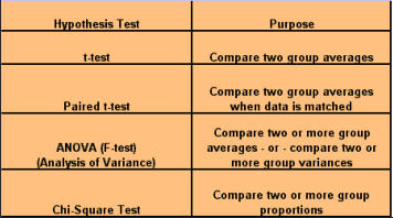
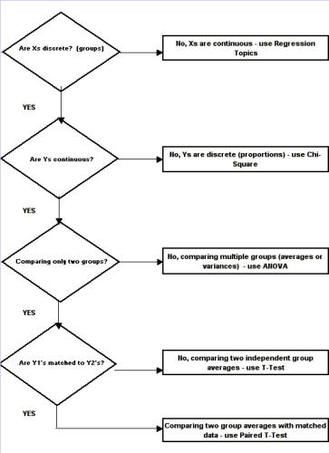
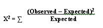
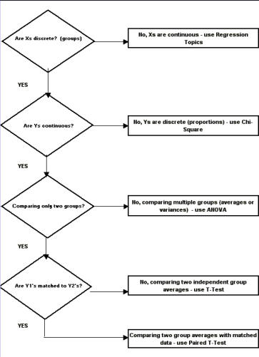
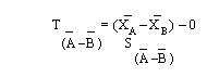
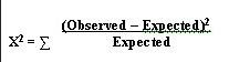
SCATTER PLOTS A scatter plot is a graph that helps you visualize the relationship between two variables. It can be used to check whether one variable is related to another and is also a good way to illustrate the relationship that may be found. I refer you to our section on scatter plots for your further information and development on this tool. Why use a scatter plot? · Studying and identifying possible relationships between the changes observed in two different sets of variables. · Understanding relationships between variables. When to use a scatter plot? · To discover whether two variables are related. · To find out if changes in one variable are associated with changes in the other. · To test for a cause-and-effect relationship (note: finding a relationship does not always indicate causation). Important notes regarding scatter plots: 1. Each data point represents a pair of measurements (for example, one dot correlates between one item on the axis versus another item on the axis. 2. Two variables are represented - generally the effect is on the vertical axis and the potential cause is on the horizontal axis. 3. Both axis are roughly equal in length, thus the plot is square. 4. The pattern formed by the scatter is an important clue to how the two variables are related, or possibly not related. 5. Stratification using different symbols allows you to look at multiple patterns at the same time. How to create a scatter plot: 1. Collect paired data along with other information. Other information could include potential stratification factors. 2. Determine which variable will be on the horizontal axis (x) and which will be on the vertical axis (y). By convention, place the potential cause on the horizontal axis and the effect on the vertical axis. 3. Find the minimum and maximum of x and y. 4. Set up the plot axis - each axis should be about the same length. 5. Plot all the x, y pairs on the graph. 6. Label the graph. To Interpret the Scatter Plot, you need to look for outliers, but the emphasis is on the main pattern formed by the scatter of the data points. The tighter together that the points are clustered, the stronger the correlation. A pattern that slopes from the lower left corner to the upper right corner means that as the variable on the X-axis increases, so does the variable on the Y-axis. This is a positive correlation. For example, if you were studying that paint tends to take longer to dry because of an increase in humidity, your scatter plot may show a positive correlation because as the humidity goes up, the time it takes for paint to dry also lengthens. A pattern than slopes from the upper left corner down to the lower right corner means that as the variable on the X-axis increases, the variable on the Y-axis decreases. This would be an inverse or negative correlation. To go back to our example earlier, a scatter plot of the order lead time vs. the number of operators available on the shift may show a negative correlation because as the number of operators goes up, the lead time goes down. Why use a scatter plot? · Studying and identifying possible relationships between the changes observed in two different sets of variables. · Understanding relationships between variables. When to use a scatter plot? · To discover whether two variables are related. · To find out if changes in one variable are associated with changes in the other. · To test for a cause-and-effect relationship (note: finding a relationship does not always indicate causation). Correlation and Causation Even strong correlations do not imply causation. If there is a pattern on your scatter plot, it doesn't necessarily mean that the two variables are related. It is likely that there is a positive correlation, but possibly not causation between the occurrences of one item to another. Conversely, no correlation does not mean also that there is no causation; there may be relationships over a wider range of data, or a different portion of the range of data. You should verify your cause review; do this by: · Selecting the most likely causes to verify. · Use existing data or collect new data to see if these causes contribute to the problem. · Use scatter plots, stratified frequency plots, tables or experimentation to understand the relationship between the causes and the effects. · You may even try doing a Hypothesis test. Hypothesis Tests A hypothesis test is a procedure that summarizes data so you can detect differences among groups. It is used to make comparisons between two or more groups. How hypothesis tests work - since there is variation, no two things will be exactly alike. The question is whether the differences you see between samples, groups, processes, etc., are due to random, common-cause variation, or if there is a real difference that exists. To help you make this decision, various hypothesis tests provide ways of estimating common cause variation for different situations. These test whether a difference is significantly bigger than the common cause variation you would expect for the situation that exists. If the answer is no, there is no statistical evidence of a difference. If the answer is yes, conclude that the groups are significantly different. Hypothesis tests take advantage of larger samples because the variation among averages decreases as the sample size increases. We will now begin to discover the power of statistical testing methods. Before we begin, there are some definitions you need to understand. H0 = no difference between groups or data sets Ha = groups are different. P value = the probability of obtaining the observed difference given that the "true" difference is zero. A hypothesis test: · Tests the "null" hypothesis (no difference between groups). · Against the alternative hypothesis (groups are different). · Obtain a P-value for the null hypothesis. · Use the data and the appropriate hypothesis; test statistic to obtain a P-value. · If P is less than .05, reject the H0 and conclude the Ha. · If P is greater than or equal to .05, cannot reject the H0. Why use a hypothesis test? · To detect differences that may be pertinent to your business. · You are unsure if minor difference in averages is due to random variation or if it reflects a true difference. When to use a hypothesis test? · When you need to compare two or more groups: on average, in variability, or in proportion. · You are not sure if a true difference exists. Assumptions for hypothesis testing - if data are continuous, we assume the underlying distribution is normal. You may need to transform non-normal data (such as cycle times). When comparing groups from different populations, you can assume: · Independent samples · Achieved through random sampling. · The samples are representative (unbiased) of the population. When comparing groups from different processes we assume: · Each process is stable. · There are no special causes or shifts over time (that is, no time-related differences). · The samples are representative of the process (unbiased). P-value definitions: · Hypothesis tests compare observed differences between groups. · The P-value equals the probability of obtaining the observed difference given that the "true" difference is zero (= the null hypothesis). · P-values range from 0.0 to 1.0 (0% chance to 100% chance). · By convention, usually treat P as less than .05 as indicative that the difference is significant. · If P is less than .05, conclude there is little chance that the true difference is 0. Referring back to the types of data, again there are two types - Discrete and Continuous: Discrete - proportions. Continuous - averages, variation, and shapes or distributions. How to use a Hypothesis Test: 1. Determine the type of test suited to your data and question. 2. Select the appropriate test. 3. Obtain p value; declare statistically significant difference if p <.05. Two types of errors in hypothesis testing There are four possible outcomes to any decision we make based on a hypothesis test - We can decide the groups are the same or different, and we can be right or wrong. Type I error - Deciding the groups are different when they aren't (the difference is due to random variation). Type II error - Not detecting a difference when there really is one. P-value - the probability of making a Type I error. You choose what level of Type I error you're willing to live with, by convention it is usually set at .05 or 5%; thus it is said there is 95% confidence level. The probability of making a type II error can be calculated given an assumed true difference. Practical Implications of type I and type II errors: · Both errors are important. · Guarding too heavily against one error increase the risk of the other error. · Increasing the sample size reduces the risk of type II errors. · Allows you to detect small differences. T-TEST We use a statistical test called the t-test for comparing and judging difference between two group averages. The formula for t is the same as for Z, but P-values are obtained from the t-distribution instead of the Z-distribution. The confidence interval A 95% confidence interval is the range of values we expect to contain the true difference between the two group averages. It's based on the "difference distribution of averages" not the differences between individual observations. It does not represent the range of values we expect for the difference between individual growth times; that range would be wider. If there is no significant difference between the group averages, the confidence level will contain 0 (that is, range from negative [ - ] to positive [ + ]. Summary of the t-test: · It is a test of hypothesis for comparing two averages. · The hypothesis is that the two group averages are the same. · Their difference = 0. · If P-value is low, <.05, reject the hypothesis. Common notation: Null hypothesis H0: meanA = meanB Alternative hypothesis HA: meanA ¹ meanB Paired T-Test Matched or paired data Two measurements are obtained for each sampling unit (a transaction, phone call, employee, deal, application, etc.) Measurements in the second group are not independent from those in the first group. They are matched or paired. The second measurements are taken on the same sampling units as the first measurements. Practical implications of Paired t-tests: · The Paired t-test is a powerful way to compare two methods. · Requires a special matched data structure. The sampling unit (machine, operation, material, etc.) needs to have each method applied to both; has little or no carryover from the use of the first method to the use of the second; requires planning; applies in the analysis or improvement stages of a project (example - you're looking to find or demonstrate a difference between two ways of running a process). ANOVA Comparing two or more group averages. ANOVA is a statistical test that uses variance to compare multiple averages simultaneously. Instead of comparing pair wise averages, it compares the variance between groups to the variance within groups. The between-group variance is obtained from the variance, or S2, of the group averages. The within-group variance is obtained from the variance S2, among values within each group, and then pooled (or averaged with appropriate differences) across the groups. If the variance between groups is the same as the variance within groups, we say there is no difference between the group averages. S2 between S2 within You need to: · Obtain the variance between groups. · Obtain the variance within groups. · If they are about the same, conclude there is no significant difference between groups. · The ratio of two variances = F-statistic. · We get a P-value from the F-distribution. Assumptions for ANOVA · The samples are representative of the population or process. · The process IS stable. · Only common causes of variation exist within the process. · No shifts or drifts/trends over time (no time-related special causes). · The variance for each group is the same. · Can be verified with the F-test · Violation of these assumptions can cause incorrect conclusions in the ANOVA analysis. · It is also assumed that the underlying distribution of each group is Normal. This can be checked with a Normal probability plot of residuals (we will cover this in the Regression section). Does the variation differ between groups? How to check: There is a statistical test called Homogeneity of Variance to check this assumption. "Homogeneity" means "the same" so actually you're testing to determine if the variances are the same. Review of ANOVA: · Used to compare averages of two or more groups. · Assumes variances of each group are the same. · Also used to compare variances of two or more groups. · Called the Homogeneity of Variance test. · Use this test to check the assumption that variances are the same when comparing averages. CHI-SQUARE This is the hypothesis test used to compare two or more group proportions. It is used when both X and Y are discrete. The counts are summarized in a table known as a contingency table. The Chi-Square measures the difference between the observed and the expected counts in this way: What Next? Determine which group proportions are different. Determine why the group proportions are different. Assumptions of the Chi-Square Test · The sample is representative of the population or process. · We assume the underlying distribution is binomial for discrete data used in a X2 test. · The expected count greater than or equal to 5 for each cell, or the test will not perform properly. · If expected count is less than 5, collecting additional data (bigger sample) is probably needed. Value of Chi-Square Test · Discrete data are commonly collected and used to analyze process performance in the service applications within manufacturing. · Non-significant differences between two or more groups keep you from chasing ghosts. · There is little to gain by studying the best or trying to motivate the worst performers. · Significant differences between group proportions can be detected. · A low P-value (less than .05) indicates that it is appropriate to identify root causes that night lead to significant differences between groups. · Examine the chi-square values for each cell to determine which groups are different. · Remember to consider whether the size of the "statistically significant" difference in proportions is actually important to the business. CONTINUE TO PART THREE OF ANALYZE NEXT- - PART THREE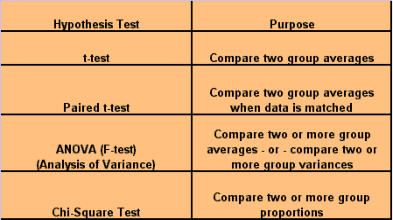


STEP #3 - ANALYZE CON’T
ORGANIZE & ANALYZE DATA

Step #3 - ANALYZE - PART 2
SCATTER PLOTS A scatter plot is a graph that helps you visualize the relationship between two variables. It can be used to check whether one variable is related to another and is also a good way to illustrate the relationship that may be found. I refer you to our section on scatter plots for your further information and development on this tool. Why use a scatter plot? · Studying and identifying possible relationships between the changes observed in two different sets of variables. · Understanding relationships between variables. When to use a scatter plot? · To discover whether two variables are related. · To find out if changes in one variable are associated with changes in the other. · To test for a cause-and-effect relationship (note: finding a relationship does not always indicate causation). Important notes regarding scatter plots: 1. Each data point represents a pair of measurements (for example, one dot correlates between one item on the axis versus another item on the axis. 2. Two variables are represented - generally the effect is on the vertical axis and the potential cause is on the horizontal axis. 3. Both axis are roughly equal in length, thus the plot is square. 4. The pattern formed by the scatter is an important clue to how the two variables are related, or possibly not related. 5. Stratification using different symbols allows you to look at multiple patterns at the same time. How to create a scatter plot: 1. Collect paired data along with other information. Other information could include potential stratification factors. 2. Determine which variable will be on the horizontal axis (x) and which will be on the vertical axis (y). By convention, place the potential cause on the horizontal axis and the effect on the vertical axis. 3. Find the minimum and maximum of x and y. 4. Set up the plot axis - each axis should be about the same length. 5. Plot all the x, y pairs on the graph. 6. Label the graph. To Interpret the Scatter Plot, you need to look for outliers, but the emphasis is on the main pattern formed by the scatter of the data points. The tighter together that the points are clustered, the stronger the correlation. A pattern that slopes from the lower left corner to the upper right corner means that as the variable on the X-axis increases, so does the variable on the Y-axis. This is a positive correlation. For example, if you were studying that paint tends to take longer to dry because of an increase in humidity, your scatter plot may show a positive correlation because as the humidity goes up, the time it takes for paint to dry also lengthens. A pattern than slopes from the upper left corner down to the lower right corner means that as the variable on the X-axis increases, the variable on the Y-axis decreases. This would be an inverse or negative correlation. To go back to our example earlier, a scatter plot of the order lead time vs. the number of operators available on the shift may show a negative correlation because as the number of operators goes up, the lead time goes down. Why use a scatter plot? · Studying and identifying possible relationships between the changes observed in two different sets of variables. · Understanding relationships between variables. When to use a scatter plot? · To discover whether two variables are related. · To find out if changes in one variable are associated with changes in the other. · To test for a cause-and-effect relationship (note: finding a relationship does not always indicate causation). Correlation and Causation Even strong correlations do not imply causation. If there is a pattern on your scatter plot, it doesn't necessarily mean that the two variables are related. It is likely that there is a positive correlation, but possibly not causation between the occurrences of one item to another. Conversely, no correlation does not mean also that there is no causation; there may be relationships over a wider range of data, or a different portion of the range of data. You should verify your cause review; do this by: · Selecting the most likely causes to verify. · Use existing data or collect new data to see if these causes contribute to the problem. · Use scatter plots, stratified frequency plots, tables or experimentation to understand the relationship between the causes and the effects. · You may even try doing a Hypothesis test. Hypothesis Tests A hypothesis test is a procedure that summarizes data so you can detect differences among groups. It is used to make comparisons between two or more groups. How hypothesis tests work - since there is variation, no two things will be exactly alike. The question is whether the differences you see between samples, groups, processes, etc., are due to random, common-cause variation, or if there is a real difference that exists. To help you make this decision, various hypothesis tests provide ways of estimating common cause variation for different situations. These test whether a difference is significantly bigger than the common cause variation you would expect for the situation that exists. If the answer is no, there is no statistical evidence of a difference. If the answer is yes, conclude that the groups are significantly different. Hypothesis tests take advantage of larger samples because the variation among averages decreases as the sample size increases. We will now begin to discover the power of statistical testing methods. Before we begin, there are some definitions you need to understand. H0 = no difference between groups or data sets Ha = groups are different. P value = the probability of obtaining the observed difference given that the "true" difference is zero. A hypothesis test: · Tests the "null" hypothesis (no difference between groups). · Against the alternative hypothesis (groups are different). · Obtain a P-value for the null hypothesis. · Use the data and the appropriate hypothesis; test statistic to obtain a P-value. · If P is less than .05, reject the H0 and conclude the Ha. · If P is greater than or equal to .05, cannot reject the H0. Why use a hypothesis test? · To detect differences that may be pertinent to your business. · You are unsure if minor difference in averages is due to random variation or if it reflects a true difference. When to use a hypothesis test? · When you need to compare two or more groups: on average, in variability, or in proportion. · You are not sure if a true difference exists. Assumptions for hypothesis testing - if data are continuous, we assume the underlying distribution is normal. You may need to transform non-normal data (such as cycle times). When comparing groups from different populations, you can assume: · Independent samples · Achieved through random sampling. · The samples are representative (unbiased) of the population. When comparing groups from different processes we assume: · Each process is stable. · There are no special causes or shifts over time (that is, no time-related differences). · The samples are representative of the process (unbiased). P-value definitions: · Hypothesis tests compare observed differences between groups. · The P-value equals the probability of obtaining the observed difference given that the "true" difference is zero (= the null hypothesis). · P-values range from 0.0 to 1.0 (0% chance to 100% chance). · By convention, usually treat P as less than .05 as indicative that the difference is significant. · If P is less than .05, conclude there is little chance that the true difference is 0. Referring back to the types of data, again there are two types - Discrete and Continuous: Discrete - proportions. Continuous - averages, variation, and shapes or distributions. How to use a Hypothesis Test: 1. Determine the type of test suited to your data and question. 2. Select the appropriate test. 3. Obtain p value; declare statistically significant difference if p <.05. Two types of errors in hypothesis testing There are four possible outcomes to any decision we make based on a hypothesis test - We can decide the groups are the same or different, and we can be right or wrong. Type I error - Deciding the groups are different when they aren't (the difference is due to random variation). Type II error - Not detecting a difference when there really is one. P-value - the probability of making a Type I error. You choose what level of Type I error you're willing to live with, by convention it is usually set at .05 or 5%; thus it is said there is 95% confidence level. The probability of making a type II error can be calculated given an assumed true difference. Practical Implications of type I and type II errors: · Both errors are important. · Guarding too heavily against one error increase the risk of the other error. · Increasing the sample size reduces the risk of type II errors. · Allows you to detect small differences. T-TEST We use a statistical test called the t-test for comparing and judging difference between two group averages. The formula for t is the same as for Z, but P-values are obtained from the t- distribution instead of the Z-distribution. The confidence interval A 95% confidence interval is the range of values we expect to contain the true difference between the two group averages. It's based on the "difference distribution of averages" not the differences between individual observations. It does not represent the range of values we expect for the difference between individual growth times; that range would be wider. If there is no significant difference between the group averages, the confidence level will contain 0 (that is, range from negative [ - ] to positive [ + ]. Summary of the t-test: · It is a test of hypothesis for comparing two averages. · The hypothesis is that the two group averages are the same. · Their difference = 0. · If P-value is low, <.05, reject the hypothesis. Common notation: Null hypothesis H0: meanA = meanB Alternative hypothesis HA: meanA ¹ meanB Paired T-Test Matched or paired data Two measurements are obtained for each sampling unit (a transaction, phone call, employee, deal, application, etc.) Measurements in the second group are not independent from those in the first group. They are matched or paired. The second measurements are taken on the same sampling units as the first measurements. Practical implications of Paired t-tests: · The Paired t-test is a powerful way to compare two methods. · Requires a special matched data structure. The sampling unit (machine, operation, material, etc.) needs to have each method applied to both; has little or no carryover from the use of the first method to the use of the second; requires planning; applies in the analysis or improvement stages of a project (example - you're looking to find or demonstrate a difference between two ways of running a process). ANOVA Comparing two or more group averages. ANOVA is a statistical test that uses variance to compare multiple averages simultaneously. Instead of comparing pair wise averages, it compares the variance between groups to the variance within groups. The between-group variance is obtained from the variance, or S2, of the group averages. The within-group variance is obtained from the variance S2, among values within each group, and then pooled (or averaged with appropriate differences) across the groups. If the variance between groups is the same as the variance within groups, we say there is no difference between the group averages. S2 between S2 within You need to: · Obtain the variance between groups. · Obtain the variance within groups. · If they are about the same, conclude there is no significant difference between groups. · The ratio of two variances = F-statistic. · We get a P-value from the F-distribution. Assumptions for ANOVA · The samples are representative of the population or process. · The process IS stable. · Only common causes of variation exist within the process. · No shifts or drifts/trends over time (no time- related special causes). · The variance for each group is the same. · Can be verified with the F-test · Violation of these assumptions can cause incorrect conclusions in the ANOVA analysis. · It is also assumed that the underlying distribution of each group is Normal. This can be checked with a Normal probability plot of residuals (we will cover this in the Regression section). Does the variation differ between groups? How to check: There is a statistical test called Homogeneity of Variance to check this assumption. "Homogeneity" means "the same" so actually you're testing to determine if the variances are the same. Review of ANOVA: · Used to compare averages of two or more groups. · Assumes variances of each group are the same. · Also used to compare variances of two or more groups. · Called the Homogeneity of Variance test. · Use this test to check the assumption that variances are the same when comparing averages. CHI-SQUARE This is the hypothesis test used to compare two or more group proportions. It is used when both X and Y are discrete. The counts are summarized in a table known as a contingency table. The Chi- Square measures the difference between the observed and the expected counts in this way: What Next? Determine which group proportions are different. Determine why the group proportions are different. Assumptions of the Chi-Square Test · The sample is representative of the population or process. · We assume the underlying distribution is binomial for discrete data used in a X2 test. · The expected count greater than or equal to 5 for each cell, or the test will not perform properly. · If expected count is less than 5, collecting additional data (bigger sample) is probably needed. Value of Chi-Square Test · Discrete data are commonly collected and used to analyze process performance in the service applications within manufacturing. · Non-significant differences between two or more groups keep you from chasing ghosts. · There is little to gain by studying the best or trying to motivate the worst performers. · Significant differences between group proportions can be detected. · A low P-value (less than .05) indicates that it is appropriate to identify root causes that night lead to significant differences between groups. · Examine the chi-square values for each cell to determine which groups are different. · Remember to consider whether the size of the "statistically significant" difference in proportions is actually important to the business. CONTINUE TO PART THREE OF ANALYZE NEXT- - PART THREE
© The Quality Web, authored by Frank E. Armstrong, Making Sense
Chronicles - 2003 - 2016